In our previous post, we began by looking at some examples of geospatial SQL, working with real data about Colombia that were loaded into CartoDB. In this post, we will continue to see spatial SQL queries and some simple examples of spatial analysis using SQL language.
Geospatial SQL and aggregated functions
Using spatial relationships along with aggregation functions and the group by grouping clause opens the way for very powerful operations with the available data. Let's begin with a simple example: The number of schools in each of the barrios in Bogota.
As shown in the previous post, this is done by entering the SQL console on the dashboard for the barrios_de_bogota table and running the following SQL query
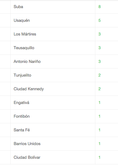
SELECT b.name, count(p.type) as hospitals FROM barrios_de_bogota b JOINpoints p on st_contains(b.geom, p.geom) WHERE p.type = 'hospital'GROUP BY b.name ORDER BY hospitals desc
The result is the list of barrios, along with the number of schools in each barrio, sorted from the highest to the lowest number of schools.
In short, the operations performed by this query are as follows:
1. The JOIN clause creates a virtual table that includes the data of the barrios and points of interest
2. WHERE filters the virtual table only for the columns where the point of interest is a hospital
3. The resulting rows are grouped by barrio name and filled in with the COUNT() aggregation function.
Geospatial analysis in CartoDB
As mentioned, the use of PostGIS spatial functions along with PostreSQL aggregation functions generates a very powerful binomial. There is also the option of performing a spatial analysis of aggregated data. As an example, we are going to see the proportional estimate of census data, using the distance between spatial elements as the criterion.
This example is based on a similar example presented in the PostGIS Cookbook. This is a recommended manual of reference for medium / advanced PostGIS users.
As a starting point, we are going to use the vector data of the barrios in Bogota and the vector data of the railroads (tables barrios_de_bogota and railroads, respectively). To see the two layers (tables) simultaneously, click on the Add Layer option at the top of the right-hand bar

Choose the railroads table as the layer
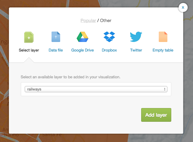
When CartoDB displays more than one layer at a time, it request permission to build a visualization. Accept and name it. The two layers are now visible at the same time.
Now, look for a railroad that crosses 3 barrios (Fontibón, Puente Aranda and Los Mártires)
Now, build a buffer zone of 1 km around that railroad. We are assuming that the people who use that railroad live at a reasonable distance from it. To do so, first exit the visualization and return to the barrios_de_bogota table. Then, run the following query from the SQL console of that table
SELECT
1 as gid,
ST_Transform(ST_Buffer(
(SELECT ST_Transform(the_geom, 21818) FROM railroads WHERE gid = 2), 1000, 'endcap=round join=round'), 4326) as the_geom
Review the documents referring to the ST_Transform function to better understand the parameters that are being used. As shown in the previous post, this function is used to specify the distances in meters (in this case, by creating a 1-km buffer zone around the line representing the railroad).
The result of this query shows a single row and, most importantly, the option of creating a table using the result
Click on the create table from query option and give it a name. In this case, railroad_buffer. Now, you are ready to create a new visualization, this time by adding another two layers. Take the same steps used to add the railroads layer previously, but this time add the layers railroads and railroad_buffer
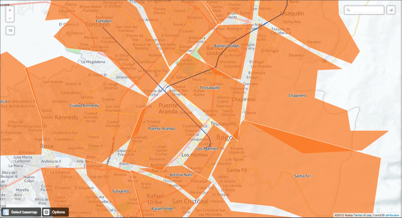
If you superimpose the table that has been created on the provinces, the following will be displayed
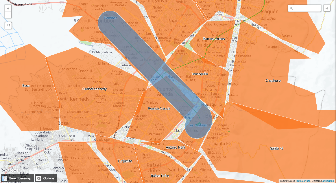
Note that there are 4 barrios that intersect with this buffer. The three barrios mentioned before, plus Teusaquillo.
A first approach to finding out the potential population that uses the railroad is simply by adding the populations of the barrios intersected by the buffer. This can be done by using the following spatial query:
SELECT SUM(b.population) as pop
FROM barrios_de_bogota b JOIN railroad_buffer r
ON ST_Intersects(b.the_geom, r.the_geom)
This first approach will yield a result of 819,892 people.
However, notice that the population is overestimated if we take into account the shape of the barrios, since all the barrios are used completely. Likewise, if we only use the barrios whose centroids intersect the buffer, the result will probably be an underestimation.
Therefore, we should assume that the population is more or less evenly distributed (this is only an approximation, but more accurate than the results we have up to now). Therefore, if 50% of the polygon representing a barrio is within the area of influence (1 km around the railroad), it can be assumed that 50% of the population of that barrio are potential users of the railroad. The estimate will be somewhat more accurate by adding these amounts for all the barrios involved. This will yield a proportional sum.
This operation is carried out by building a function in PL/pgSQL. This function can be called up in a query, just like any other PostGIS spatial function. Copy this code in the SQL console of the barrios_de_bogota table, as usual
CREATE OR REPLACE FUNCTION public.proportional_sum(geometry, geometry, numeric)
RETURNS numeric AS
$BODY$
SELECT $3 * areacalc FROM
(
SELECT (ST_Area(ST_Intersection($1, $2))/ST_Area($2)):: numeric AS areacalc
) AS areac;
$BODY$
LANGUAGE sql VOLATILE
As arguments, this function uses the two geometric elements to intersect and the total number of the population for which we want to obtain the proportional population that will use the railroad. It returns the estimated number. The operation simply consists in multiplying the proportion in which the barrios overlap the area of interest by the amount to be proportioned (the population).
The function is called up as follows:
SELECT ROUND(SUM(proportional_sum(a.the_geom, b.the_geom, b.population))) FROM
railroad_buffer a, barrios_de_bogota b
WHERE ST_Intersects(a.the_geom, b.the_geom)
GROUP BY a.cartodb_id
In this case, the result is 248,217, which seems more reasonable.

This exercise marks the end of our series of posts on geospatial SQL. In the first post of the series, we gave a theoretical introduction on spatial predicates and the geospatial index concept. The second post dealt with a series of simple examples using these predicates and specific geographic data pertaining to Colombia. This third post has shown how to use the aggregated functions applied to spatial queries and a simple spatial analysis exercise. In all the examples, we have used CartoDB, the easiest way to use a spatial database without having to install any software in our computer.